A jökulhlaup from a Laurentian captured ice shelf to the Gulf of Mexico could have caused the Bølling warming

Abstract

Since the rapid rate of the global warming at the onset of Bølling became evident, its cause has been under debate. It coincides closely in time with a strong global transgression called meltwater pulse 1a (mwp-1a). One attempt of solution says that an mwp-1a of Antarctic origin could cause an increase in North Atlantic Deep Water (NADW) formation, and thus give rise to the Bølling interstadial. However, others have disputed that Antarctic meltwater would have that effect, and furthermore, the start of Bølling is not even associated with an increase in NADW. A controversial hypothesis says that some Laurentian meltwater came from a sub-glacial jökulhlaup, but no study yet has shown unequivocally that sufficient amounts of water could be stored under the ice. Furthermore, according to all available data a meltwater pulse from the Laurentian ice gives rise to strong cooling, not warming. Nevertheless, megafloods appear instrumental in accumulating the Mississippi Fan, created entirely during the Quaternary period, and dramatic climate changes are characteristic of our period. This paper presents an hypothetical chain of events, building on the published literature and simple calculations to see if the order of magnitude is reasonable. The hypothesis is that a jökulhlaup from a Laurentian captured ice shelf (CIS) flowed out through the Mississippi, boosted the Gulf Stream, reinvigorated the North Atlantic circulation, and as a result triggered the Bølling warm phase.

Introduction

Ice core records indicate that the temperature rose very quickly during deglaciation, and most abruptly at the onset of the Bølling warm phase around 14 600 BP (Fig. 1; unless otherwise noted all times are in calendar years). Studies of reef crest corals show that the world sea level rose dramatically on several occasions during deglaciation (Fairbanks 1989, Blanchon and Shaw 1995), and most dramatically in meltwater pulse 1a (mwp-1a). It now appears clear that mwp-1a was synchronous with the onset of Bølling (Kienast et al. 2003).

Weaver et al. (2003) concluded that an hypothetical mwp-1a of Antarctic origin could cause an increase in North Atlantic Deep Water (NADW) formation, and thus give rise to the Bølling interstadial. However, Seidov et al. (2005) disputed that Antarctic meltwater would have that effect on NADW, and furthermore, McManus et al. (2004) concluded that NADW had in fact not increased. Instead, they suggested that the warming led to the melting, and that they happened in that order. Then again, this does not explain the warming, nor does the warming provide enough energy for the rapid melting.

Throughout the ice age the temperature was able to rise more abruptly than it fell, in what is known as Dansgaard-Oeschger (D/O) events. The enigma of what causes the sudden warming applies to D/O events as well as for the start of Bølling and Holocene.

On the other hand, evidence abounds for a connection between large freshwater discharges to the North Atlantic, and cooling. The inter-Allerød 400-year cold spell around 13 100 BP has been correlated with the catastrophic drainage of Glacial Lake Iroquois through the Hudson River Channel (Donnelly et al. 2005). Another cold anomaly was triggered when glacial Lake Candona was drained towards Gulf St. Lawrence (Broecker et al. 1989, Donnelly et al. 2005). Drainage of Lake Agassiz to the Mackenzie River caused a short-duration cooling early in Holocene (Fisher et al. 2002), and the final drainage of Lake Agassiz through Hudson Strait has been connected with the 8200 BP cold event (Clark et al. 2004). All of these are consistent with model results showing that meltwater pulses to the North Atlantic are capable of causing sudden cooling (e.g. Ganapolski and Rahmstorf 2001), but never warming.

In spite of this evidence, since meltwater pulses from the Antarctic can apparently be ruled out as explanation, the Laurentian ice sheet remains the only potential source of mwp-1a. The solution of the enigma might therefore be to find a mediatory process that can convert a freshwater pulse to a warm climatic event. A few recent research results are of special interest since they in combination might explain what caused mwp-1a and Bølling, and by extension also other events.

The first is described in Erlingsson (2006), who successfully tested the captured ice shelf (CIS) hypothesis (Erlingsson 1994a, 1994b) on Lake Vostok in the East Antarctic. Recently Alley et al. (2005) reinvented the hypothesis while providing additional arguments based on the heat budget. Applying the CIS hypothesis to the Laurentian ice sheet provides a source of the water for the required continental-scale jökulhlaup.

The second result is Aharon (2006), who showed that mwp-1a was associated with a large hyperpycnal flow to the Gulf of Mexico, and that this turbidity current preceded the dilution peak of the surface waters. In fact, there may have been two or even three closely spaced turbidity currents.

The final one is McManus et al. (2004), who showed that the onset of Bølling was associated with a sudden and strong increase in the meridional overturning circulation (MOC), without any change in NADW (Fig. 2). They studied a proxy in a core from the Bermuda rise, and found a large increase in sedimentation rate simultaneous with the onset of the MOC. The Bermuda rise is of course located downstream from the Gulf of Mexico in terms of surface currents and the MOC. Heinrich event 1 (H1), preceding Bølling during Oldest Dryas, was marked by a virtual shut down of NADW-formation by icebergs and freshwater dilution (incidentally Alley et al. 2005 hypothesized that H1 was caused by a jökulhlaup from a CIS in Hudson Bay).

Hypothesis

The following hypothetical scenario for the Bølling warming is presented. A large captured lake existed under a CIS stretching from Hudson Bay and almost down to the Great Lakes (Fig. 3). A jökulhlaup released a very large amount of water in a rather short time towards the Gulf of Mexico. It provided a burst of water to the Gulf, the volume of which was significant in relation to the yearly volume of the contemporary Gulf Stream. The duration was less than the residence time of the Loop Current.

The flood entered the Gulf of Mexico as a turbidity current. When it had shed the sediments it got mixed and rose, but not all the way to the surface. Instead it created a new intermediate layer. The rapid increase of volume in the Gulf of Mexico forced out warm and saline surface water before the newly arrived cold fresh water reached the threshold (it is argued that this was a transient situation that did not follow the rules of steady-state circulation).

The effect was a strengthened Gulf Stream, without a correspondingly large dilution or cooling of the waters leaving the Florida Strait. This caused the observed increase in sedimentation at Bermuda, according to the hypothesis, and the Bølling warm phase.

Evaluation

Discharge

As a way of testing if the hypothesis is consistent with field data, the water and sediment discharge will be compared with available information, side effects of canyon erosion will be examined, and the feedback mechanism on the climate will be looked into. This requires that the CIS jökulhlaup be quantified.

A jökulhlaup from a captured lake like the one in Figure 3 may have had a volume of 10¹⁴ m³. Even if the flow rate equalled 10⁶–10⁷ m³s^-1  when leaving the ice, in analogy with the Alberta data, the hydrograph would have been smoothened in the Mississippi valley. Large areas would have been inundated, and there is also a possibility for ice dams along the way, increasing the area of flooding even more. When the flow reached the sea the maximal discharge is therefore expected to have been in the lower part of that range. The following calculations are based on an hypothetical flow of 10⁶ m³s^-1 during 3 years, thus in the lower end of the estimated range.

Paleoflow

We may convert published estimates for flow rate to flow volume, since the jökulhlaup duration was much shorter than the residence time of the Gulf of Mexico. However, a complication is that most flow rates are based on data from above the thermocline. The volume in the Gulf was at this time about 2.2 10¹⁵ m³, but mixing did not necessarily involve the whole water mass.

Multiplying 33 years with 0.110⁶ m³s^-1—0.2310⁶ m³s^-1, the estimated flow rate of Emiliani et al. (1978), yields total fresh water volumes that are 104% and 240%, respectively, of the hypothetical jökulhlaup volume. However, two factors may make the estimated volume an underestimate. First, the assumption of Emiliani et al. (1978) that the relationship between peak flow and mean annual runoff was the same then as now is obviously invalid if a jökulhlaup was involved. Secondly, when calculating the residence time they assumed that “[n]o export of deep water is possible because formation of such water is inhibited by the permanent thermocline.” However, they apparently overlooked the possibility that intermediate water, composed of mixed turbidity current water and deep water, is exported to the Caribbean Sea through the Yucatan Channel, and is replaced by the import of new deep water the same way. This water exchange seems an inevitable result of the turbidity currents, since the mixing during mwp-1a did not reach the surface according to Aharon (2006). In fact, it might be this intermediate layer that Haddad and Droxler (1996) detected in the Caribbean Sea. Taking this into account, the d¹⁸O data comfortably allow for a jökulhlaup of 10¹⁴ m³.

The discharge estimate of Aharon (2006) is similarly irrelevant in the light of a CIS jökulhlaup hypothesis. At best, we can adopt it to an order of magnitude by making some changes. Assume first that all the water was derived from the captured lake, and that the d¹⁸O value of –25‰ reported by Remenda et al. (1994) is representative for the subglacial water. This would lower the discharge estimate to 0.1110⁶ m³s^-1, which obviously is unrealistically low since some of the flow would have been from rain and snowmelt, thus raising the d¹⁸O. If accumulated over a period of 33 years, the residence time in the Gulf of Mexico assumed by Emiliani et al. (1978), this amounts to 1.1 10¹⁴ m³, which is nearly the same as the volume of the presumed jökulhlaup. Note that the temporal resolution of the core data of Aharon (2006) does not allow us to determine if a major part of the freshwater entered during a fraction of the 33 year period, or evenly distributed over the whole time interval. Furthermore, just as with the estimate of Emiliani et al. (1978), the possibility of a venting to the Caribbean Sea in the lower part of the thermocline makes the estimate very much a minimum, rather than a central estimate. In conclusion, the d¹⁸O data are clearly consistent with a jökulhlaup of 10¹⁴ m³.

Turbidity current

The required suspended sediment concentration can be calculated to less than 5% by weight. Given a sediment density of 2600 kgm^-3, a water volume of 10¹⁴ m³, and an average porosity of 40% for the turbidite deposit (based on core 615 in O’Connor et al. 1985), the volume of the resulting deposit calculates to 3.310¹² m³. Beyond doubt the last lobe of the Mississippi Fan contains significantly more sand and silt than required to drive the hypothetical jökulhlaup down to the sea floor as a turbidity current. In total, the 8 sequences of the Pleistocene fan contain enough sediment for about a hundred such jökulhlaups (cf. Fig. 4).

As regards the discharge rate into the Gulf deep waters, the capacity of the canyon can be crudely estimated as follows, using an equation for the turbidity current head velocity from Huppert and Simpson (1980). The equation gives the head height, while the turbidity current body is about half as high. A depth of 2000 m is used, a sea salinity of 35‰, and a temperature of 4 ºC for both water masses. Assuming an effective canyon width of 1.3 km, a flow of 10⁶ m³s^-1 with 5% sediment concentration yields a body height of 200 m, and a propagation velocity of 3.7 ms^-1. This would easily fit in the canyon, and furthermore, both larger and faster turbidity currents are known from the recent past (Posamentier and Walker, in press). Assuming that the average velocity was 2 ms^-1, and that 80% of the flow is outside the channel (above and beside; see e.g. Posamentier and Kolla, 2003), also the mid-fan channel could have accommodated a flow of 10⁶ m³s^-1.

The source of the sediment could include erosion under the ice lobe, and erosion of loess and flood plain deposits outside the ice margin. In conclusion, the hypothetical turbidity current from the jökulhlaup is perfectly within the realm of known processes.

Oceanographic consequences

Having seen that a meltwater pulse of 10¹⁴ m³ with a flow rate of 10⁶ m³s^-1 is possible, the question is what would happen with the water in the Gulf of Mexico, and what would the implications be for the Gulf Stream and, by extension, the climate. The series of interactions that are inferred are as follows (see Fig. 5b): (1) The turbidity current reaches the basin floor. (2) The sand is deposited, and the fresh water starts rising. (3) Under mixing, the water rises to its equilibrium depth, which is in the thermocline. (4) The new intermediate water may flow south through the Yucatan Channel (4a), and new salt deep water may be added the same way (4b). (5) The addition of water raises the sea surface elevation. (6) This leads to an increased outflow through the Florida Strait (again, this is a transient effect, and the ultimate equilibrium is not believed to be relevant in this case).

The dashed lines in Figure 5a suggest a potential stratification in the Loop Current during the jökulhlaup. This is a proxy based on modern stratification—the pycnocline during the ice age was arguably somewhat shallower (relative the contemporary water surface). Due to the shallow depth of the Florida Strait (ca 600 m), surface water will dominate the outflow. The character of the Gulf Stream water could therefore have remained rather stable, but its volume would have increased, so that the net effect might have been an increase in the energy flux to the North Atlantic.

The addition of 10⁶ m³s^-1 during 3 years might seem like a small change compared to the normal strength of the Gulf Stream during the LGM, 2010⁶ m³s^-1 (Lynch-Stieglitz et al. 1999). However, the MOC had been completely shut down during H1 (McManus et al. 2004), why even a small increase represented a significant change. Furthermore, the peak discharge might have been an order of magnitude larger, as argued above. Also, when the MOC was shut down during H1 more heat stayed in the Gulf, thus increasing the surface water temperature there by >3 ºC (Flower et al. 2004), why 10⁶ m³s^-1 represented a greater heat flux than during LGM. Finally, there may have been several closely spaced such jökulhlaups within a few centuries, since there are 2 or 3 peaks in the d¹⁸O (Aharon 2006).

In contrast, in order to boost the NADW the Gulf Stream first and foremost needs to have a high salinity. Even though the main dilution of the surface waters in the Gulf happened after the main meltwater pulse, a slight dilution is probably inevitable, and such a signal appears in core EN32-PC6 (at the arrow in Fig. 6). Since the formation of NADW is very sensitive to dilution of the water, no increase in NADW is to be expected. This is consistent with observations, indicating a strong increase in MOC but no change in NADW formation (McManus et al. 2004).

Atmospheric gases

This hypothetical chain of events seems to provide a plausible explanation for the sudden warming of Bølling. It might also suggest an explanation for the methane curve.

Simultaneously with the two most prominent rises in temperature in Greenland, the methane concentration suddenly rose (Fig. 6). The D/O events appear to show the same pattern of simultaneous rise in temperature and methane (Chappellaz et al. 1993). The methane may have come from methane hydrate, which exists under the frozen tundra and on shelf slopes.

Methane hydrate is only stable under high pressure (tens of atmospheres) and low temperatures (Dickens and Quinby-Hunt 1994). It may thus become unstable so that methane is released due to a pressure decrease or a temperature increase. Underwater methane hydrate would tend to become more stable as the sea level was rising. It has therefore been suggested that the methane increase is due to release from under the thawing permafrost.

However, another possibility is that the methane was released from the seabed by physical action. The shelf slope by the Mississippi Canyon contains methane hydrate, which makes canyon erosion a feasible mechanism for methane release. The methane hydrate there is believed to form where natural gas seeps out from petroleum reservoirs. The most straightforward hypothesis is therefore perhaps that the methane came from natural gas that leaked out when the erosion of the Mississippi Canyon penetrated a reservoir. If so, then the main canyon erosion events can be predicted to have occurred at 14.6 kBP and 11.5 kBP, with possible incipient erosion at 15.5 kBP (Fig. 6).

At the onset of Bølling also the CO₂ level goes up in the GRIP core. An hypothetical scenario can be sketched as follows: An oil field was penetrated by the jökulhlaup when creating the Mississippi Canyon. Large amounts of natural gas—consisting largely of methane—bubbled up. Being lighter than air it ascended violently, creating atmospheric turbulence that built up electric charges. When they discharged in the form of lightening and thunder, oil on the sea surface was ignited. This scenario is consistent with the methane and carbon dioxide data, as well as with the release of isotopically old carbon (something that is implied by a bend in the ¹⁴C calibration curve of Reimer et al. 2004).

Incidentally, the geology of the outer Louisiana shelf at the upper part of the canyon contains a significant amount of tabular salt intrusions (Diegel et al. 1995). If salt was dissolved when canyons were eroded it would have increased the salinity and density of the inflowing water. Note that it would not have affected the isotopic composition of the seawater, why the mixed water would have appeared diluted in the d¹⁸O data regardless of what salinity it actually had. Although an analysis of 3D seismic data covering the most recent canyon found no indication of erosional contact with salt, it can not be ruled out entirely as a potentially contributing factor.

Other climate events

So far the focus has been on the process that caused mwp-1a and the onset of Bølling. Having identified a chain of events that may have happened on more than one occasion, it may be discussed what other events in the geologic record could have been partly or entirely caused by this process.

The onset of Bølling coincided with a withdrawal of the southern Laurentian ice margin as shown in Figure 8b, which represents changes during time interval b in Figure 6. The withdrawal may represent dead ice ablation following a jökulhlaup. A similar withdrawal event happened during time interval a (Fig. 8a), although the methane concentration rose much less, and there is no real net effect in the temperature (Fig. 6). Still, also event a might have been a jökulhlaup. The lack of a clear temperature signal could be an effect of the small volume, and perhaps that the tendencies to create warming and cooling cancelled out.

Figure 8c reflects the event when an ice lobe in Lake Superior temporarily dammed Lake Agassiz thus causing a drainage event to the Mississippi, and then melted off in timeframe g in Figure 6. This coincides with a sudden rise in methane (Fig. 6) and in sea level (Fig. 1). Neither event a nor g led to a rapid start of MOC (Fig. 2); during a MOC remained off, and when g happened the MOC was already recuperating after having been only partially shut off during Younger Dryas by a process similar to the one that provoked H1. However, McManus et al. (2004) caution that the resolution is inadequate, so also Younger Dryas might have been caused by a complete shutdown of MOC followed by a rapid restart.

Neither event a nor g gave rise to strong hyperpycnal flows according to the data of Aharon (2006). However, it is possible that such a flow occurred, but that the mixing stayed at a too low level for detection (the deepest core is from 529 m below the present sea level), especially if the inflowing water picked up salt on the slope. Therefore it can not be ruled out that the sudden warming at the start of Holocene at least partially was influenced by turbidity currents to the Gulf of Mexico, although there may as yet be no evidence for it.

Returning to Bølling, it was followed by Older Dryas, which coincided with the peak of the meltwater dilution of the surface waters of the Gulf (letter c in Fig. 6). In this case the cause and effect appears straightforward: meltwater to the surface leads to cooling. During Allerød the methane level remains high, while both Greenland temperature and d¹⁸O in the Gulf decrease stepwise. It seems possible that the period was marked by recurring turbidity currents that left little impact neither on the surface d¹⁸O nor on the North Atlantic temperature, but that they eroded the canyon thus releasing methane, and that they contributed to the development of the Mississippi Fan. The source may have been marginal lake drainages.

The D/O events are marked by the same sudden increase in temperature and methane, followed by a slow return. Thus, both the ice cores on Greenland, and the geology of the Mississippi Fan hint that this process may have been repeated many times, and may hav e been one of the main factors in provoking sudden climate change during the Quaternary. While it has been proposed that sudden cooling may be caused by a jökulhlaup from a CIS through Hudson Strait (Alley et al. 2005), it may thus be that sudden warming can be caused by a jökulhlaup from a CIS through the Mississippi.

If these speculations regarding other hypothetical jökulhlaups and turbidity currents are correct, it follows that what made mwp-1a appear in cores near the surface was the size of it. The other events would have mixed out in the lower half of the thermocline, i.e. at 600 to 1200 m below the present sea level. The study of Haddad and Droxler (1996) possibly found this water. If so, a comparison of their record with the size of the Laurentian ice sheet ought to show a correlation between the intermediate water type and the position of the southern ice margin. Having said this, it is obvious that many other factors, including the wind and the sea level, also affect the outcome in complex webs of cause and effect.

It should be noted that this hypothesis does not necessarily affect the estimate of the maximal volume of the Laurentian ice sheet. The lowest sea level, -125 m, occurred 22–19 kBP (Yokoyama et al. 2000), but by the onset of mwp-1a the sea level had already risen some 30 m. The difference between a grounded traditional inland ice, and the profile with a large captured ice shelf present, could be equivalent to a sea level change of as little as 10 to 15 m. Perhaps counter-intuitively, a CIS does not require a thin floating ice since—as the Lake Vostok case shows—the air temperature largely governs the thickness. Thus, even if the CIS during the LGM was diminished to small lakes like those now found under the Antarctic, and the ice volume was as large as that suggested by Peltier (2004), it may still be possible that an extensive CIS could have been formed by the onset of Bølling and give rise to the jökulhlaup suggested above.

Conclusion

A hypothesis has been presented for how a megaflood from the Laurentian inland ice could have been responsible for the Bølling warming through a chain of events, many of which seem to have support in geological data. Furthermore, the evaluation suggests that this may not have been an exception, but a defining criterion of the Pleistocene climate. Having said this, it must be added that the hypothesis has only been evaluated preliminarily; it has yet to be tested properly.

It seems likely that a jökulhlaup from a captured lake under the Laurentian ice sheet entered the Gulf of Mexico as a turbidity current, thus forcing out warm surface water into the Gulf Stream, which restarted the MOC in the North Atlantic, which in turn caused the Bølling warm phase. The trigger for the jökulhlaup could be any combination of internal glacial dynamics and climate forcing. Although the discharge rate of the jökuhlhlaup may have been less than the Gulf Stream during LGM, it had a strong effect since it appeared at a time when the MOC was turned off (having been shut down by H1) and the Gulf surface waters were warm. It may be added that it would make no difference for the end result if the water instead came from the drainage of marginal Lake Agassiz, as long as the discharge and sediment concentration were large enough.

The Gulf Coast contains vast petroleum reserves. It is arguably very likely that gas and oil was released when the Mississippi Canyon was formed. This might be the source of the increased atmospheric methane concentration recorded in the Greenland ice core at the start of Bølling and Holocene.

This chain of events may have acted in a similar way at the end of each major Laurentian glaciation, and possibly also at D/O events. Geological data suggests that it has been repeated at least eight, possibly a hundred times, all in the Pleistocene. It may play a decisive role in bringing about the sudden climate changes that are so characteristic of the Quaternary period, as well as in creating the Mississippi Fan.

Noting that the Laurentian CIS jökulhlaups discussed in this paper may explain sudden warming, and that the Laurentian CIS jökulhlaups discussed by Alley et al. (2005) may explain the sudden cooling of Heinrich events, it follows that the existence and behaviour of a Laurentian captured ice shelf may be crucial for question of the Quaternary climate.

References

Abascal, A.J., Sheinbaum, J., Candela, J., Ochoa, J., and Badan, A., 2003: Analysis of flow variability in the Yucatan Channel. Journal of Geophysical Research, 108 (C12): 11-1.

Aharon, P., 2006: Entrainment of meltwaters in hyperpycnal flows during deglaciation superflows in the Gulf of Mexico. Earth and Planetary Science Letters, 241: 260-270.

Alley, R.B., Dupont, T.K., Parizek, B.R., Anandakrishnan, S., Lawson, D.E., Larson, G.J. and Evenson, E.B., 2005: Outburst flooding and the initiation of ice-stream surges in response to climatic cooling: A hypothesis. Geomorphology 75:76-89.

Beaney, C. L. and Shaw, J., 2000: The subglacial geomorphology of southeast Alberta: evidence for subglacial meltwater erosion. Can. J. Earth Sci., 37:51-61.

Blanchon, P. and Shaw, J., 1995: Reef drowning during the last glaciation: evidence for catastrophic sea-level rise and ice sheet collapse. Geology, 23:4–8.

Bond, G., Heinrich, H., Broecker, W., Labeyrie, L., McManus, J., Andrews, J., Huon, S., Jantschik, R., Clasen, S., Simet, C., Tedesco, K., Klas, M., Bonani, G. and Ivy, S., 1992: Evidence for massive discharges of icebergs into the North Atlantic ocean during the last glacial period. Nature 360: 245-249.

Bond, G., Showers, W., Cheseby, M., Lotti, R., Almasi, P., deMenocal, P., Priore, P., Cullen, H., Hajdas, I. And Bonani, G., 1997: A Pervasive Millennial-Scale Cycle in North Atlantic Holocene and Glacial Climates. Science, 278(5341): 1257-1266.

Bouma, A.H., Stelting, C.E., and Coleman, J.M., 1985: Mississippi Fan, Gulf of Mexico. In Submarine fans and related turbidite systems, Bouma, A.H., Normark, W.R. and Barnes, N.E., (Eds.). Springer, New York.

Brennand, T.A., Russel, H.A.J., and Sharpe, D.R., 2003: Tunnel channels of central

 southern Ontario: character, genesis and glaciodynamic implications. Paper presented at the XVI INQUA Congress, Reno, Nevada, USA, 23—30 July 2003.

Broecker, W.S., Kennett, J.P., Flower, B.P., Teller, J.T., Trumbore, S., Bonani, G. and Wolfli, W., 1989: Routing of meltwater from the Laurentide Ice Sheet during the Younger Dryas cold episode. Nature, 341: 318-321.

Bunge, L., Ochoa, J., Badan, A., Candela, J., and Sheinbaum, J., 2003: Deep flows in the Yucatan Channel and their relation to dhanges in the Loop current extension. Journal of Geophysical Research, 108 (C12): 26-1.

Candela, J., Tanahara, S., Crepon, M. and Barnier, B., 2003: The Yucatan Channel flow: Observations vs. CLIPPER ATL6 and MERCATOR models. Journal of Geophysical Research 108 (C12):

Chappellaz, J.A., Bluniert, T., Raynaud, D., Barnola, J.M., Schwander, J. and Stauffert, B., 1993: Synchronous changes in atmospheric CH4 and Greenland climate between 40 and 8 kyr BP. Nature 366: 443-445.

Clark, C.D.  and Stokes, C.R., 2001: Extent and basal characteristics of the M’Clintock Channel Ice Stream. Quaternary International 86: 81-101.

Clark, G.K.C., Leverington, D.W., Teller, J.T. and Dyke, A.S., 2004: Paleohydraulics of the last outburst flood from glacial Lake Agassiz and the 8200 BP cold event. Quaternary Science Reviews, 23: 389-407.

Denton, G.H. and Karlén, W., 1973: Holocene climatic variations—Their pattern and possible cause. Quaternary Research 3(2): 155-174.

Dickens, G.R. and Quinby-Hunt, M.S., 1994: Methane hydrate stability in seawater. Geophysical Research Letters 21(19): 2115-2118.

Diegel, F.A., Karlo, J.F., Schuster, D.C., Shoup, R.C. and Tauvers, P.R., 1995: Cenozoic structural evolution and tectonostratigraphic framework of the northern Gulg Coast continental margin. In Salt Tectonics: a Global Perspective, Jackson, M.P.A., Roberts, D.G. and Snelson, S. (Eds.). American Association of Petroleum Geologists Memoir, 65: 109-151.

Donnelly, J.P., Driscoll, N.W., Uchupi, E., Keigwin, L.D., Schwab, W.C., Thieler, E.R. and Swift, S.A., 2005: Catastrophic meltwater discharge down the Hudson Valley: A potential trigger for the Intra-Allerød cold period. Geology 33(2): 89-92.

Dyke, A.S., Moore, A. and Robertson, L., 2003: Deglaciation of North America. Geological Survey of Canada, Open File 1574.

Emiliani, C., Gartner, S., Lidz, B., Eldridg, K., Elvøy, D.K., Huang, T.C., Stipp, J.J. and Swanson, M.F., 1975: Paleoclimatological analysis of late Quaternary cores from the northeastern Gulf of Mexico. Science 189: 1083-1088.

Emiliani, C., Rooth, C. and Stripp, J.J., 1978: The late Wisconsin flood into the Gulf of Mexico. Earth and Planetary Science Letters 41(2): 159-162.

Erdoes, R. and Ortiz, A., 1985: American Indian Myths and Legends. Pantheon.

Erlingsson, U., 1994a: The ‘Captured Ice Shelf’ hypothesis and its applicability to the Weichselian glaciation. Geografiska Annaler 76A (1–2): 1–12.

—1994b: A computer model along a flow-line of an Ice Dome—‘Captured Ice Shelf’. Geografiska Annaler 76A (1–2): 13–24.

—2006: Lake Vostok behaves like a ‘captured lake’ and may be near to creating an Antarctic jökulhlaup. Geografiska Annaler 88A (1): 1–7.

Fairbanks, R.G., 1989: A 17,000-year glacio-eustatic sea level record: influence of glacial melting rates on the Younger Dryas event and deep-ocean circulation. Nature, 342: 637-642.

Fisher, T.G., Smith, D.G. and Andrews, J.T., 2002: Preboreal oscillation caused by a glacial Lake Agassiz flood. Quaternary Science Reviews 21: 873-878.

Flower, B.P., Hastings, D.W., Hill, H.W. and Quinn, T.M., 2004: Phasing of deglacial warming and Laurentide Ice Sheet meltwater in the Gulf of Mexico. Geology, 32: 597–600.

Ganapolski, A. and Rahmstorf, S., 2001: Rapid changes of glacial climate simulated in a coupled climate model. Nature 409: 153–158.

GRIP Members, 1993: Climate instability during the last interglacial period recorded in the GRIP ice core. Nature 364: 203-207.

Haddad, G.A. and Droxler, A.W., 1996: Metastable CaCO₃ dissolution at intermediate water depths of the Caribbean and western North Atlantic: Implications for intermediate water circulation during the past 200,000 years. Paleoceanography, 11(6): 701-716.

Heinrich, H., 1988: Origin and consequences of cyclic ice rafting in the Northeast Atlantic Ocean during the past 130,000 years. Quarternary Research 29: 143–152.

Huppert, H.E. and Simpson, J.E., 1980: The slumping of gravity currents. Journal of Fluid Mechanics, 99: 785-799.

Keigwin, L.D., Jones, G.A., Lehman, S.J., and Boyle, E.A., 1991: Deglacial Meltwater Discharge, North Atlantic Deep Circulation, and Abrupt Climate Change. Journal of Geophysical Research 96 (C9): 16811-16826.

Kennett, J.P. and Shackleton, N.J., 1975: Laurentide ice sheet meltwater recorded in Gulf of Mexico deep-sea cores. Science 188: 147-150.

Kienast, M., Hanebuth, T.J.J., Pelejero, C. and Steinke, S., 2003: Synchroneity of meltwater pulse 1a and the Bølling warming: new evidence from the South China Sea. Geology, 31: 67-70.

Kolla, V. and Perlmutter, M.A., 1993: Timing of turbidite sedimentation on the Mississippi Fan. American Association of Petroleum Geologists Bulletin 77: 1129-1141.

Kor, P. S. G., Shaw, J. and Sharpe, D. R., 1991: Erosion of bedrock by subglacial meltwater, Georgian Bay, Ontario: a regional view. Canadian Journal of Earth Sciences 28: 623–642.

Leventer, A., Williams, D.F. and Kennett, J.P., 1982: Dynamics of the Laurentide ice sheet during the last deglaciation: evidence from the Gulf of Mexico. Earth and Planetary Science Letters 59(1): 11–17.

Lynch-Stieglitz, J., Curry, W.B. and Slowey, N., 1999. Weaker Gulf Stream in the Florida Straits during the Last Glacial Maximum. Nature 402: 644-648.

McManus, J.F., Francois, R., Gherardi, J.M., Keigwin, L.D., and Brown-Leger, S., 2004: Collapse and rapid resumption of Atlantic meridional circulation linked to deglacial climate changes. Nature, 428: 834-837.

Mulder, T. and Syvitski, J.P.M., 1995: Turbidity currents generated at river mouths during exceptional discharges to the world oceans. Journal of Geology, 103(3): 285-299.

Ochoa, J., Sheinbaum, J., Badan, A., Candela, J. and Wilson, D., 2001: Geostrophy via potential vorticity inversion in the Yucatan Channel, Journal of Marine Research, 59: 725–747.

O’Connell, S., Stelting, C.E., Bouma, A.H., Coleman, J.M., Cremer, M., Droz, L., Meyer-Weight, A.A., Normark, W.R., Pickering, K.T., Stow, D.A.V., and DSDP Leg 96 Shipboard Scientists, 1985: Drilling Results on the Lower Mississippi Fan. In Submarine fans and related turbidite systems, Bouma, A.H., Normark, W.R. and Barnes, N.E., (Eds.). Springer, New York.

Peltier, W.R., 2004: Global Glacial Isostacy and the Surface of the Ice-Age Earth: The ICE5G (VM2) Model and GRACE. Annual Review of Earth and Planetary Sciences, 32: 111–149.

Posamentier, H.W. and Kolla, V., 2003: Seismic geomorphology and stratigraphy of depositional elements in deep-water settings. Journal of Sedimentary Research, 73: 367-388.

Posamentier, H.W. and Walker, R.G., 2006: Deep-water turbidites and submarine fans. In: Posamentier, H.W. and Walker, R.G. (Eds.), Facies Models Revisited (CD). SEPM Special Publications, ISBN 1565761219.

Reimer, P.J., Baillie, M.G.L., Bard, E., Bayliss, A., Beck, J.W., Bertrand, C.J.H., Blackwell, P.G., Buch, C.E., Burr, G.S., Cutler, K.B., Darnon, P.E., Edwards, R.L., Fairbanks, R.G., Friedrich, M., Guilderson, T.P., Hogg, A.G., Hughen, K.A., Kromer, B., McCormac, G., Manning, S., Ramsey, C.B., Reimer, R.W., Remmele, S., Southon, J.R., Stuiver, M., Talamo, S., Taylor, F.W., van der Plicht, J. and Weyhenmeyer, C.E., 2004: IntCal04 Terrestrial Radiocarbon Age Calibration, 0–26 cal kyr BP. Radiocarbon, 46: 1029–1058.

Remenda, V.H., Cherry, J.A. and Edwards, T.W.D., 1994: Isotopic composition of old groundwater from Lake Agassiz: implications for late Pleistocene climate. Science, 266: 1975–1978.

Roberts, M.J., 2005: Jökulhlaups: a reassessment of floodwater flow through glaciers. Reviews of Geophysics, 43(RG1002): 1-21.

Seidov, D., Stouffer, R.J. and Haupt, B.J., 2005: Is there a bi-polar ocean seesaw? Global and Planetary Change, 49: 19-27.

Shaw, J., 1983: Drumlin formation related to inverted melt-water erosional marks. J. Glaciol., 29:461–479.

Shaw, J., Rains, B., Eyton, R. and Weissling, L., 1996: Laurentide subglacial outburst floods: landform evidence from digital elevation models. Canadian Journal of Earth Sciences 33:1154–1168.

Shoosmith, D.R., Baringer, M.O. and Johns, W.E., 2005: A continuous record of Florida Current heat transport at 27°N. Geophysical Research Letters 32(23), doi:10.1029/2005GL024075.

Tarasov, L. and Peltier, W.R., 2005: Arctic freshwater forcing of the Younger Dryas cold reversal. Nature, 435: 662-665.

Yokoyama, Y., Lambeck, K., de Deckker, P., Johnston, P. and Fifield, L.K., 2000: Timing of the Last Glacial Maximum from observed sea-level minima. Nature, 406: 713-716. Correction 2001, Nature, 412: 99.

Weaver, A.J., Saenko, O.A., Clark, P.U. and Mitrovica, J.X., 2003: Meltwater pulse 1A from Antarctica as a trigger of the Bølling-Allerød warm interval. Science, 299(5613): 1709-1713.

Figure 1. Temperature proxy from the GRIP ice core (GRIP Members 1993; time scale ss09) covering the last two ice age terminations. The solid line is the d¹⁸O from 15 to 6 cal kBP (bottom abscissa, left ordinate), dashed line is d¹⁸O from 144 to 130 cal kBP in the same core (top abscissa, left ordinate), representing the transition from Saale to Eem. The dash-dot line is an inferred sea level curve from the last deglaciation (bottom abscissa, right ordinate; from Blanchon and Shaw, 1995). The first sudden rise represents mwp-1a.

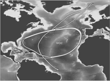
Figure 2. Sketch of the North Atlantic currents. Deep water (NADW) is formed north of Iceland in Holocene, by sinking of cold and saline water. The meridional overturning circulation (MOC) was shut down during Heinrich event 1 and increased suddenly at the start of Bølling, but in contrast NADW did not increase (McManus et al. 2004).

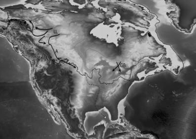
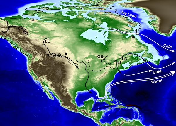
Figure 3. The Wisconsin glaciation. Solid line marks the glaciation limit. Bold solid arrows mark identified jökulhlaups (LL=Livingston Lake, A=Alberta, GB=Georgian Bay). Dashed arrow marks the extramarginal continuation through the Missouri and the Mississippi Rivers, and the Mississippi Canyon and Fan. The dotted line outlines the hypothetical captured lake. The map reflects a –70 m sea level without isostatic adjustment.

Figure 4. The Gulf of Mexico and northern Caribbean Sea at LGM, ca 20 kBP. The present-day course of the Gulf Stream is shown, with the characteristic Loop Current in the Gulf of Mexico. White dots outline the Mississippi Fan. The black arrow shows the path of the Mississippi River and the last channel on the Mississippi Fan. A: location of sediment core EN32-PC6, B: location of oceanographic station 681463, F: Florida Strait, H: Hispaniola, Y: Yucatan Channel.

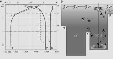
Figure 5. Key oceanographic factors of the Gulf of Mexico. (a) Water stratification at location B in Fig. 4. S: salinity, T: temperature, r: density. Solid lines are modern measurements from the month of May in the Loop Current (NODC accession number 7500019), dashed lines are hypothetical profiles explained in the section “Evaluation”. The dotted line W is the ice age water level. (b) Length section along the Gulf Stream (white arrows) from the entrance to the Caribbean Sea (CS) at Hispaniola (H), further through the Yucatan Channel (Y) to the Gulf of Mexico (GOM) with its loop current, and out through the Florida Strait (F). Numbered arrows are discussed in the section “Evaluation”.

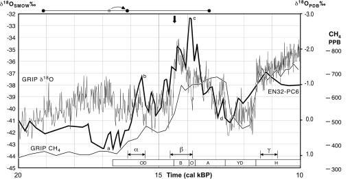
Figure 6. Temperature proxy and methane content (Chappellaz et al. 1993) in the GRIP ice core, compared to d¹⁸O data for Globigerinoides ruber in the Orca Basin (core EN32-PC6; for location see A in Fig. 4), from Leventer et al. (1982, Figs. 1, 3). The age model of the core is based on Keigwin et al. (1991), although the point at 16.9 kBP has been moved to 16.1 kBP with hinge points at 19.2 and 13.2 kBP, to compensate for assumed increased sedimentation rate when the meltwater flow drastically increased (the line with dots above the diagram illustrates the move). The arrow marks a 28 cm thick non-laminated layer that Leventer et al. (1982, p. 13) interpreted as having been “rapidly redeposited from shallow depths during a period of intense melt-water discharge.” With this age model it is synchronous with mwp-1a. Keigwin et al. (1991) defined the four peaks a through d. The intervals a through g mark periods when ice lobes melted away (see Fig. 8). OD=Oldest Dryas (with Heinrich event 1), B=Bølling, O=Older Dryas, A=Allerød, YD=Younger Dryas, H=Holocene.

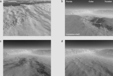
Figure 7. Virtual photos of the Mississippi Fan. (a) View from the south with sea level at -120 m. M: Latest canyon.  S: Salt nappe cut through by an older canyon. (b) View from above the latest canyon. (c) View down the upper fan. (d) View down the middle fan. The latest channel complex can be seen veering off to the left. The images were created from ETOPO-2 elevation data in the software Terragen with 20 times vertical exaggeration.

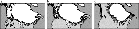
Figure 8. Deglaciation events during the Wisconsin ice age. The bold line marks the ice margin at the end of each time interval. Arrows mark meltwater routes. Data from Dyke et al. (2003). The calendar year conversion is done using Reimer et al. (2004). (a) 16.1 – 15.35 kBP (13.5 – 13 ¹⁴C kBP). (b) 14.7 – 13.85 kBP (12.5 – 12 ¹⁴C kBP). (c) 11.4 – 10.85 kBP (10 – 9.6 ¹⁴C kBP). The time intervals are illustrated in Fig. 6, a, b, and g, respectively.

---

Background

This appendix is supplied as an aid to those readers who may not be familiar with results from the various fields that are involved. Hopefully it will also be useful for understanding what considerations the hypothesis is based on.

Climate changes

The dramatic climate warming around 14.7 ka BP must be considered together with the normal climatic fluctuations during the ice age. Although the Holocene climate seems to fluctuate with a period of ~1,500 years (Denton and Karlén 1973, Bond et al. 1997), the variations during the last ice age were much larger (Bond et al. 1997, Ganapolski and Rahmstorf 2001) as shown by analyses of d¹⁸O in ice cores from Greenland (GRIP Members 1993, Chappellaz et al. 1993). The pattern of D/O events is a sudden warming followed by a gradual return to full glacial conditions. These interstadials seem to become rare towards the pleniglacial.

During the ice age there were also phases of extreme cold associated with Heinrich events, when ice-rifted material from the Hudson Strait Ice Stream reached far southeast in the North Atlantic Ocean (Heinrich 1988, Bond et al. 1992). They occur more seldom (5–10 ka) and with less regularity than D/O events, during phases that already are cold. The temperature on Greenland did not fall much from its already cold state, but on the European Atlantic coast these stadials brought severe cooling.

Ganapolski and Rahmstorf (2001) suggested oceanographic explanations for both these types of events. During glaciations, North Atlantic Deep Water (NADW) is normally formed south of Iceland, whereas it forms north of Iceland during interglacial periods. They concluded that there was a latch effect in the glacial system, and that the normal cold phase suddenly could shift to warm interstadial D/O conditions. The cause could be, they wrote, a small decrease in freshwater influx (10⁴ m³ s^-1) or an increase in evaporation (5ºC higher temperature), each leading to an increase in salinity.

Conversely, Heinrich events were found to represent unstable shutdowns of the NADW formation, caused by a large influx of freshwater or icebergs (>10⁵ m³ s^-1). In the model, both the Heinrich and D/O circulation patterns spontaneously returned to the normal glacial conditions within centuries after the forcing mechanism was gone.

Gulf of Mexico meltwater pulses

Leventer et al. (1982) presented d¹⁸O data from foraminifera in the anoxic Orca Basin. They identified two strong negative d¹⁸O excursions (b and c in Fig. 6), indicating two peaks in meltwater dilution of the surface waters of the Gulf. Negative anomalies in foram d¹⁸O are thought to reflect warmer water (0.23‰ d¹⁸O per °C), or a dilution of the seawater with fresh water. In this case the dilution explanation was preferred (Emiliani et al. 1978, Leventer et al. 1982, Keigwin et al. 1991).

Mg/Ca thermometry data from Orca Basin cores (Flower et al. 2004) indicate that the sea surface temperature in northern Gulf of Mexico increased steeply by >3ºC from about 17.2 to 15.5 kBP. This accounts for almost half of the d¹⁸O change from the maximum to the negative peak b in Figure 6, which leaves peak c as the main negative peak. Keigwin et al. (1991) compared this core to cores from all over the North Atlantic, and identified also two positive excursions (a and d), interpreted to represent high-latitude meltwater pulses.

The d¹⁸O of fresh water mainly reflects the temperature when the precipitation fell (‰ d¹⁸O = 0.695T – 13.6). Jökulhlaup waters will therefore have strong negative d¹⁸O values. Kennett and Shackleton (1975) assumed an isotropic composition of –30‰ for Laurentide meltwater (equivalent to –24°C) and calculated that surface seawater (–10 m) was diluted by over 8%. They also concluded that the water between –100 and –200 m was diluted by over 4%. Emiliani et al. (1975) assumed an isotropic composition of –15‰ (equivalent to –2°C) and consequently calculated twice the dilution, based on a 2.4‰ change in d¹⁸O over the secular trend.

Laurentian jökulhlaups

It has long been the dominating opinion that drumlins, Rogen moraines and similar streamlined morphology in the glacial sediments have been formed directly by the ice at its base. However, it has been proposed (Shaw 1983, Shaw et al. 1996) that at least some of them were caused by jökulhlaups. Shaw et al. (1996) estimated that 8.4 10¹³ m³ was discharged in one event at Livingston Lake (Fig. 3). The water was deflected south to the Mississippi via the Missouri, but also north to the Mackenzie River. Geological evidence indicates that the sub-glacial flow started as sheet flow but later became canalized.

Others have suggested that at least some drumlins were created not by a jökulhlaup, but by an ice stream (Clark and Stokes 2001). Some ice streams were immediately followed by a jökulhlaup, while others (such as the M’Clintock Channel ice stream) simply froze in their movement. They all contributed to a rapid decrease of the inland ice sheet volume, though, and their duration was on the order of a few centuries.

Bedrock erosion by very large subglacial flows has also been inferred in the southern parts of the Laurentian ice sheet, in eastern Alberta, directly downstream from the Livingston Lake event. The water apparently followed the foot of the Rocky Mountains towards the southern ice margin. The maximal flow has been estimated by Beaney and Shaw (2000) to 1–10 Sv  (1 sverdrup = 10⁶ m³ s^-1; not to be confused with the SI unit sievert), and the timing to no later than the onset of deglaciation.

An event with the same maximal discharge has been identified in Georgian Bay, Ontario, resulting in erosion and polishing of the crystalline bedrock (Kor et al. 1991). Recently, a number of tunnel valleys leading to Lake Ontario have been mapped (Brennand et al. 2003). They were interpreted as caused by jökulhlaups followed by stagnation, thus explaining also the surrounding dead ice morphology.

The hydrograph of modern Icelandic jökulhlaups rise either exponentially over a matter of weeks, or linearly over a matter of hours or days (Roberts 2005). The larger the jökulhlaup, the more likely the hydrograph is to rise rapidly, a behaviour thought to correspond to sheet flow from the front. Large ice blocks frequently get entrained in the flow, eroding the front of the ice lobe.

Caribbean Sea oceanography

The Gulf Stream flows through the Caribbean Sea, and enters the Gulf of Mexico as the Loop Current (Fig. 4). The deep-water characteristics are determined by the threshold level to the Atlantic, which is at ca –1600 m (Fig. 5). Atlantic water (mostly upper NADW) enters the Caribbean Sea at that level, creating virtually homogenous conditions down to the largest depths. Since the threshold in the Yucatan Channel is at –2040 m, the Gulf of Mexico receives the same deep water (there are also some local effects in the Gulf due to the presence of salt leaks).

Haddad and Droxler (1996) concluded that the CaCO₃ dissolution pattern in the Bahamas inter island deep channels and on the Nicaragua rise shifts between ice ages and interglacial periods. In the Bahamas they observed preservation in interglacial periods, and dissolution during ice ages. In the Caribbean Sea they observed the exact reverse pattern at depths below –1200 m. However, in the interval –1000 to –1200 m the situation sometimes resembled the Bahamas record, and sometimes the Caribbean >1200 m record.

Gulf Stream

The flow of the Gulf Stream in the Florida Strait is today about 30 Sv, while it during the Late Glacial Maximum (LGM) can been estimated to about 20 Sv (Lynch-Stieglitz et al. 1999, McManus et al. 2004). The average temperature is 19.37 ºC (Shoosmith et al. 2005), equivalent to the temperature at about 200 to 250 m depth.

In the Yucatan Channel the surface current has been estimated to 24 ± 4.6 Sv at present (Ochoa et al. 2001). The modern day net flow in the Yucatan Channel is to the north at levels down to the 6°C isotherm at ca 800 m depth (Candela et al. 2003), corresponding to the conditions at the threshold in the Florida Strait east of Miami (-730 m). Below that level the flows are weak and the net flow is negligible, the variability being dominated by passing eddies (Abascal et al. 2003) or compensation for the variability in the Loop Current (Bunge et al. 2003).

Mississippi palaeoflow

A palaeoflow calculation was made by Emiliani et al. (1978). They estimated that the average flow in the Mississippi River during the peak of deglaciation was 0.1–0.23 Sv, based on a residence time of 33 years for the Gulf of Mexico surface waters, and a dilution of the “entire water column” of 5–10%. This implies turbidity currents to the basin floor, although they did not explicitly say so. They further assumed that the peak discharge had the same relation to the annual maximum discharge as it has at present in the Mississippi River, and estimated the peak to 0.2–0.5 Sv.

Aharon (2006) concluded that the flow from 14.7-14.2 kBP was hyperpycnal (i.e. turbidity currents), and had a discharge of 0.28-0.33 Sv. The estimate is based on certain assumptions that are invalid if a jökulhlaup was involved, most importantly that the flow was in static equilibrium with the Loop Current.

Tarasov and Peltier (2005) modelled the meltwater from the Laurentian ice sheet, and estimated that the peak flow to the Gulf of Mexico during mwp-1a was 0.165 ± 0.025 Sv. The model did not allow for a CIS or jökulhlaups.

Turbidity currents

Turbidity currents can be generated not only by submarine screes, but also by river discharge if the fresh water is sufficiently sediment laden (Mulder and Syvitski 1995). The ability to keep sediment in suspension down the continental rise and over the basin floor is a function of velocity, and the velocity is a function of sediment concentration, creating a positive feedback loop that increases its ability to erode a canyon. When the flow reaches the basin floor it can follow a leveed channel for hundreds of kilometres. The channel is often meandering within a channel complex delimited by its own levees, so that it perhaps may be conceptually likened to a flood plain.

Finer fractions are shed since the flow is higher and wider than the channel. Eventually, when the levee height is insufficient to confine the basal sand-rich part of the flow, the flow is spread out forming a frontal splay or lobe (Posamentier and Walker, in press).

The Mississippi Canyon

During the end of the ice age the Mississippi River attached directly to a canyon, which continues out in the Mississippi Fan (Bouma et al. 1985). They estimated the eroded volume to 1.5 – 2 10¹² m³. At the lower end of the canyon, sediment cores brought up well-sorted gravel from the base of the deposits (O’Connell et al. 1985). Since the modern Mississippi is incapable of transporting that fraction, the find reveals that exceedingly extreme flows occurred when the canyon was active (Kolla and Perlmutter, 1993). Furthermore, the Mississippi is incapable of producing hyperpycnal flows at present (Mulder and Syvitski 1995).

The present canyon was likely cut during the last glaciation and filled during the most recent deglaciation. The erosion reached a depth of ca 1.1 km, and the width at the base was about 1 km. Modern 3D seismic data reveals that it likely is filled in with Holocene mass transport deposits, leaving only a ca 200 m deep and 11 km wide channel on the present-day slope (H. Posamentier, pers. comm. 2006; Fig. 7a, b).

The Mississippi Fan

The fan covers an area of over 3 10¹¹ m², and has a volume of at least 2.9 10¹⁴ m³. It consists of 8 different stages, each with its own canyon and fan lobe (Bouma et al. 1985). All 8 stages are Pleistocene in age. The last two are from the Wisconsin glaciation.

On the middle fanlobe (Fig. 7d) the channel is 2-4 km wide, and 25-45 m deep (Bouma et al. 1985). Turbidity currents follow the channel over the submarine fan as long as the heavy sand-carrying core fits entirely within the levees (Posamentier and Kolla 2003). The deposition of the sand (fine sand and silt) takes place in fanlobes of the lower fan, after the turbidity current first sheds much of the finer fractions.

O’Connell et al. (1985) described sediment core 615, from the latest fanlobe some 600 km from the shelf break. The last of the two Wisconsin sequences consisted of 220 m dominated by sand (ca 41%), while the previous one consisted of 255 m of which an estimated 64% was sand. The sand appeared in up to 10 m thick beds, and was interleaved with silts, silty muds (or silt-laminated muds), and clays and muds. This fanlobe has an area in the order of 3 10¹⁰ m².